Import packages
Here we load in Python packages designed to work with NIfTI data:
pydicomreads DICOM filesNiBabelreads and converts between NIfTI and several other common neuroimaging file formats, including ANALYZE, and can convert DICOM series to NIfTINiLearnis primarily designed to provide statistical analysis and machine learning tools for neuroimaging data. However, it also provides a number of utilities for reading and writing NIfTI images, and working with and visualizing data
As well we’ll load SciPy’s ndimage package, and Matplotlib
import pydicom
import nibabel as nib
from nibabel.nicom import dicomreaders
import nilearn as nil
from nilearn import plotting
from nilearn import image
import scipy.ndimage as ndi
import matplotlib.pyplot as plt
import os
import glob
import numpy as np
/var/folders/nq/chbqhzjx5hb6hfjx708rh2_40000gn/T/ipykernel_87894/3226889895.py:3: UserWarning: The DICOM readers are highly experimental, unstable, and only work for Siemens time-series at the moment
Please use with caution. We would be grateful for your help in improving them
from nibabel.nicom import dicomreaders
We will use NiBabel’s DICOM reader to convert the structural MRI images we worked with in the previous lesson from DICOM to NIfTI. NiBabel can read a directory of DICOM files and convert them to NIfTI format. We’ll use glob to find all DICOM files in the directory, then use NiBabel to read them and save as a compressed NIfTI file.
Here we will first list the contents of the data folder, then perform the conversion, and then list the contents again to see the new NIfTI file:
os.listdir('data')['.DS_Store',
'BIDS',
'4_sag_3d_t1_spgr.nii.gz',
'anatomical_aug13_001.hdr',
'Anat001.20040930.145131.5.T1_GRE_3D_AXIAL.0099.dcm',
'brain_scan.nii.gz',
'anatomical_aug13_001.img',
'DICOM']The files we want are in the DICOM sub-folder of the data folder. The first thing we’ll do is read these in and save all the images in an array.
# Read DICOM files and sort by slice location
dicom_files = sorted(glob.glob('data/DICOM/*.dcm'))
slices = []
slice_locations = []

for path in dicom_files:
    ds = pydicom.dcmread(path)
    slices.append(ds.pixel_array)
    slice_locations.append(ds.SliceLocation)

# Sort by slice location and stack into 3D volume
sorted_idx = np.argsort(slice_locations)
volume = np.stack([slices[i] for i in sorted_idx], axis=0)
Next we need to read the header information from the first DICOM file to get the affine matrix that describes the orientation of the images.
# Get DICOM metadata from first slice
ds = pydicom.dcmread(dicom_files[sorted_idx[0]])
orientation = np.array(ds.ImageOrientationPatient).reshape(2, 3)
position = np.array(ds.ImagePositionPatient)
pixel_spacing = ds.PixelSpacing
slice_spacing = ds.SliceThickness

# Construct affine matrix
# Row and column direction cosines from DICOM orientation
row_dir = orientation[0]  # [0, 1, 0]
col_dir = orientation[1]  # [0, 0, -1]
slice_dir = np.cross(row_dir, col_dir)  # [1, 0, 0]

affine = np.array([
    [-slice_dir[0] * slice_spacing, 0, 0, position[0]],
    [0, 0, col_dir[2] * pixel_spacing[1], position[1]],
    [0, -row_dir[1] * pixel_spacing[0], 0, position[2]],
    [0, 0, 0, 1]
])

print(f"Volume shape: {volume.shape}")
print(f"\nAffine matrix:\n{affine}")

# Create and save NIfTI image
nifti_img = nib.Nifti1Image(volume, affine)
nib.save(nifti_img, 'data/brain_scan.nii.gz')
print(f"\nSaved to: data/brain_scan.nii.gz")
Volume shape: (184, 256, 256)
Affine matrix:
[[ 1. 0. 0. 93.3994]
[ 0. 0. -1. -178.036 ]
[ 0. -1. 0. 97.0647]
[ 0. 0. 0. 1. ]]
Saved to: data/brain_scan.nii.gz
Saved to: data/brain_scan.nii.gz
So the new converted file is brain_scan.nii.gz
Load NIfTI file
We use NiBabel to read in the NIfTI file we just created. This is technically unnecessary here since we could have just used the NIfTI object created during the conversion step. However, often you might convert DICOM to Nifti with one script, and then use another script for analysis which reads in previously-created Nifti files.
# Reload and store for use in notebook
brain_vol = nib.load('data/brain_scan.nii.gz')
View metadata
We can view the image’s header by printing it (note that due to how the NiBabel Nifti1Image object is coded, we need to print() the header rather than just asking for it as a property):
print(brain_vol.header)<class 'nibabel.nifti1.Nifti1Header'> object, endian='<'
sizeof_hdr : 348
data_type : np.bytes_(b'')
db_name : np.bytes_(b'')
extents : 0
session_error : 0
regular : np.bytes_(b'')
dim_info : 0
dim : [ 3 184 256 256 1 1 1 1]
intent_p1 : 0.0
intent_p2 : 0.0
intent_p3 : 0.0
intent_code : none
datatype : int16
bitpix : 16
slice_start : 0
pixdim : [-1. 1. 1. 1. 1. 1. 1. 1.]
vox_offset : 0.0
scl_slope : nan
scl_inter : nan
slice_end : 0
slice_code : unknown
xyzt_units : 0
cal_max : 0.0
cal_min : 0.0
slice_duration : 0.0
toffset : 0.0
glmax : 0
glmin : 0
descrip : np.bytes_(b'')
aux_file : np.bytes_(b'')
qform_code : unknown
sform_code : aligned
quatern_b : -0.70710677
quatern_c : 0.0
quatern_d : 0.0
qoffset_x : 93.3994
qoffset_y : -178.036
qoffset_z : 97.0647
srow_x : [ 1. 0. 0. 93.3994]
srow_y : [ 0. 0. -1. -178.036]
srow_z : [ 0. -1. 0. 97.0647]
intent_name : np.bytes_(b'')
magic : np.bytes_(b'n+1')
Access data in the NIfTI object
NiBabel’s handling of the NIfTI format data is not quite as elegant as what we saw in the previous lesson. Rather than being able to access the data directly by referencing the name of the object (in this case, brain_vol), we need to use the method get_fdata() to do this (the “f” in this method name stands for “floating point”, as this is the type of data it returns). We will assign the result of this to a new variable so that it’s easy to work with.
brain_vol_data = brain_vol.get_fdata()
type(brain_vol_data)numpy.ndarrayWe see that the data is a familiar NumPy array, and below we see the dimensions are identical to what we saw for this image in the previous lesson:
brain_vol_data.shape(184, 256, 256)Visualize a slice
We can use .plt.imshow() as in the previous lesson:
plt.imshow(brain_vol_data[96], cmap='bone')
plt.axis('off')
plt.show()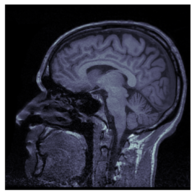
Plot a series of slices
fig_rows = 4
fig_cols = 4
n_subplots = fig_rows * fig_cols
n_slice = brain_vol_data.shape[0]
step_size = n_slice // n_subplots
plot_range = n_subplots * step_size
start_stop = int((n_slice - plot_range) / 2)

fig, axs = plt.subplots(fig_rows, fig_cols, figsize=[10, 10])

for idx, img in enumerate(range(start_stop, plot_range, step_size)):
    axs.flat[idx].imshow(brain_vol_data[img, :, :], cmap='gray')
    axs.flat[idx].axis('off')

plt.tight_layout()
plt.show()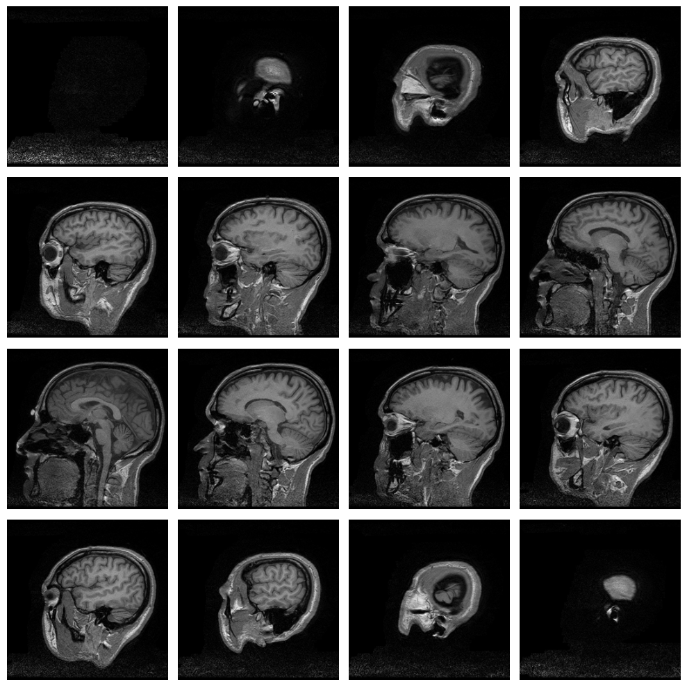
Plot with NiLearn
While SciPy’s ndimage module was designed for working with a wide variety of image types, NiLearn was designed to work with neuroimaging data specifically. As such, it’s tools are a bit easier to use and more purpose-built for tasks that neuroimaging data scientists might want to perform. For example, we can plot the NiBabel NIfTI image object directly without first having to extract the data, using the plot_img() function from NiLearn’s plotting module:
plotting.plot_anat(brain_vol)
plt.show()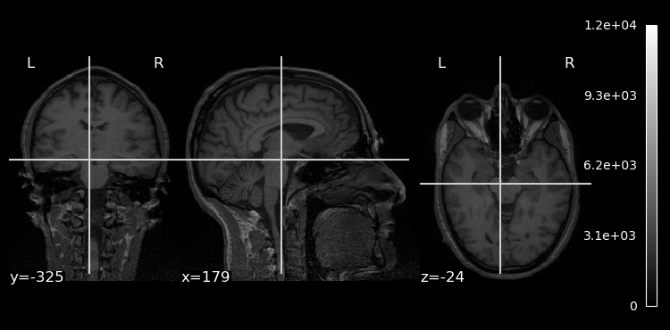
One nice thing that we see is that since NiLearn is neuroimaging-aware, it explicitly adds labels to our plot showing us clearly which the left and right hemispheres are.
NiLearn’s plotting library uses Matplotlib, so we can use familiar tricks to do things like adjust the image size and colormap:
fig, ax = plt.subplots(figsize=[10, 5])
plotting.plot_img(brain_vol, cmap='gray', axes=ax, radiological=False)
plt.show()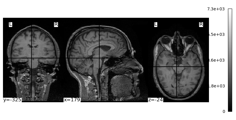
The plot_img() function also provides a variety of ways to display the brain, with much less code than we had to use when working with raw NumPy arrays and Matplotlib functions:
plotting.plot_img(brain_vol, display_mode='tiled', cmap='gray', radiological=False)
plt.show()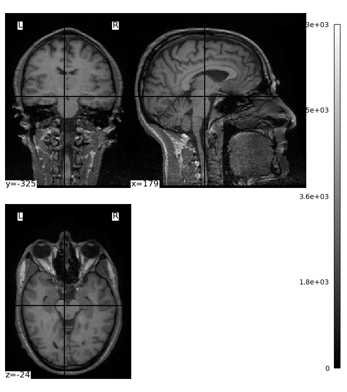
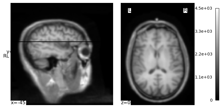
We can use the cut_coords kwarg to specify there to centre the crosshairs and “cuts” through the image that we visualize. In this image, the coordinates are relative to the *isocenter of the MRI scanner — the centre of the magnetic field inside the scanner. The position of a person’s head relative to this isocenter will vary from individual to individual, and scan to scan, due to variations in head size and the optimizations used by the MRI technician and scanner. But we can use the coordinates printed in the above image (which defaulted to the centre of the image volume) and some trial-and-error to get a different view through the brain:
plotting.plot_img(brain_vol, cmap='gray', cut_coords=(-45, 40, 0), radiological=False)
plt.show()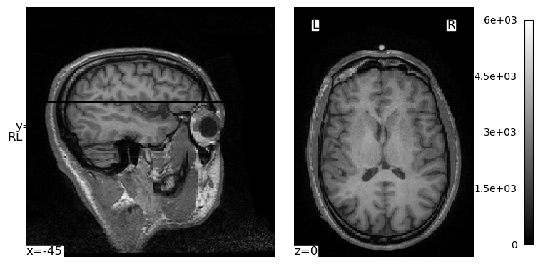
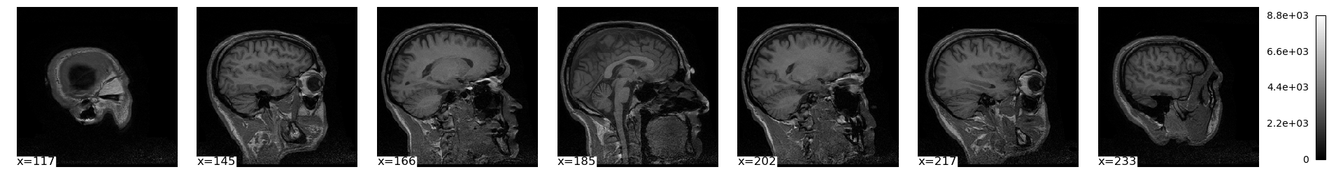
plot_img() also has a few other ways to see multiple slices at once:
plotting.plot_img(brain_vol, display_mode='x', cmap='gray', radiological=False)
plt.show()
/var/folders/nq/chbqhzjx5hb6hfjx708rh2_40000gn/T/ipykernel_87894/210350123.py:1: UserWarning: A non-diagonal affine is found in the given image. Reordering the image to get diagonal affine for finding cuts in the slices.
plotting.plot_img(brain_vol, display_mode='x', cmap='gray', radiological=False)
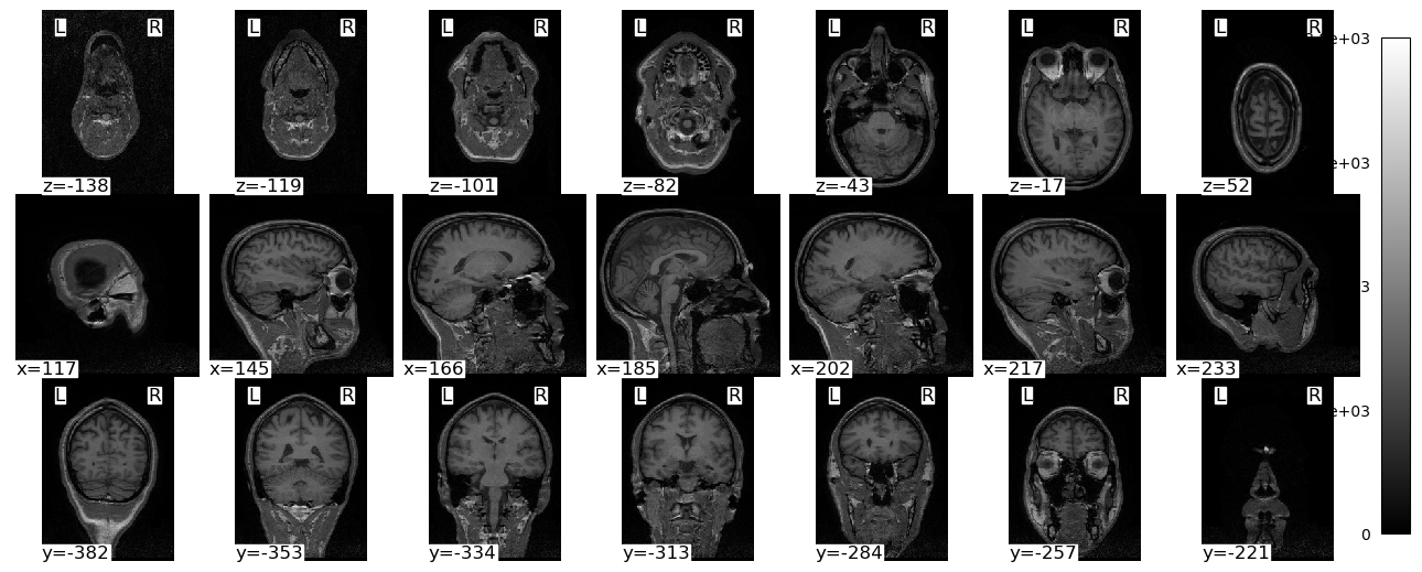
plotting.plot_img(brain_vol, display_mode='mosaic', cmap='gray', radiological=False)
plt.show()
/var/folders/nq/chbqhzjx5hb6hfjx708rh2_40000gn/T/ipykernel_87894/2634030509.py:1: UserWarning: A non-diagonal affine is found in the given image. Reordering the image to get diagonal affine for finding cuts in the slices.
plotting.plot_img(brain_vol, display_mode='mosaic', cmap='gray', radiological=False)
Smoothing
NiLearn has its own function for applying Gaussian spatial smoothing to images as well. The only real difference from scipy.ndimage’s gaussian_filter() function is that instead of specifying the smoothing kernel in standard deviations, we specify it in units of full width half-maximum (FWHM). This is the standard way that most neuroimaging analysis packages specify smoothing kernel size, so it is preferable to SciPy’s approach. As the term implies, FWHM is the width of the smoothing kernel, in millimetres, at the point in the kernel where it is half of its maximum height. Thus a larger FWHM value applies more smoothing.
fwhm = 4

brain_vol_smth = image.smooth_img(brain_vol, fwhm)
plotting.plot_img(brain_vol_smth, cmap='gray', cut_coords=(-45, 40, 0), radiological=False)
plt.show()