Spreadsheets

A wide variety of software packages and platforms are used in data science. You have probably worked with some of these in the past. Spreadsheets provide a graphical user interface (GUI) that allows the user to enter data into a table, which is composed of individual cells organized into rows and columns. Cells can contain different types of data, like numbers, letters, words, and sentences. Cells can also contain more complex data, like equations that calculate values, often based on data contained in other cells. Spreadsheets can be used to create visualizations of data, such as graphs, and perform simple statistical analyses, such as t-tests.

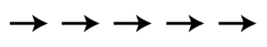
Spreadsheets are useful tools for quickly inspecting data, and manually entering data if you need to do that. However, they are limited in many ways. To illustrate some of these limitations, let’s take a simple example. Imagine you ran a simple behavioral reaction time (RT) experiment, called a “flanker” task. In this experiment, participants had to press either the left or right arrow key, to indicate whether an arrow shown on the screen is pointing left or right, respectively. However, the catch is that the centre arrow is “flanked” by two other arrows on each side; these can be pointing the same way as the target arrow (congruent):

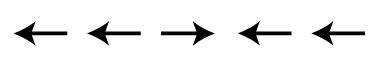
or in the opposite direction (incongruent)

We expect that the incongruent condition would be associated with slower RTs, because the flanking arrows create some visual confusion and response competition (cognitive interference; this process is not unlike that underlying the famous Stroop experiment, which you are likely familiar with). In order to confirm this hypothesis, we would want to get an estimate of the RT for each condition, from a representative sample of human participants. We need a number of participants because we know that there is variability in the average RT from person to person (between-subject variability). For our example, let’s say we tested 40 participants.

To estimate the average RT for each condition for an individual, we would want to present many trials of each condition, in random order. We do this because there is always some trial-to-trial variability in measuring human RTs (within-subject variability). We might want to include 50 trials per condition.

We normally run experiments like this on a computer, which would save a data file for each participant. So at the end of data collection, you now have a 40 data files; one from each participant. An example data file is shown in the figure below, showing the first 10 trials for one participant (identified as subj_01) as it might appear in Microsoft Excel.

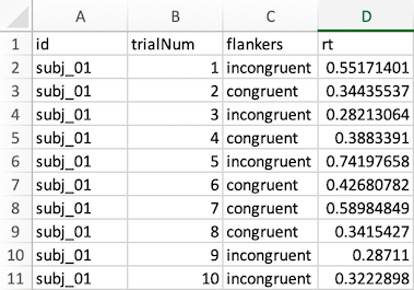
In this file, each row represents a trial, except for the first row, which is the header that labels each column. Each data row (numbered 2-11 in the spreadsheet) contains columns identifying the participant; the trial number, the condition (congruent or incongruent), and the RT (in seconds).

Since our goal is to estimate the average RT for each condition, we could use Excel’s AVERAGE function for this. However, we can’t simply put the formula =AVERAGE(D2:D101) below the bottom row (remember, we ran 100 trials, even though only the first 10 are shown in the example above). This would give us the average RT for that participant, but would not provide separate RTs for each condition. Since the conditions are randomly intermixed, calculating the RT for each condition is actually a bit challenging. However, we could use Excel’s “sort” function to sort the data by column C, which would result in all the congruent trials coming first, and the incongruent ones after. Then, we could insert two AVERAGE formulas, one for each condition.

Since in our example we tested 40 participants, we would have to manually perform this process 40 times: open a data file, sort by column C, type in two formulas, and computer the average RTs for each condition. Then we would copy and paste these into a new spreadsheet, that had one row and two columns (mean congruent RT, mean incongruent RT) for each subject. Once we had done this 50 times, we could use Excel’s AVERAGE function again to compute the mean RT across participants for each condition. To please our stats teacher, we might also compute the standard deviation (a measure of variability) across the subjects, which would be another equation put in another cell.

Note

There is nothing fundamentally incorrect with this process, and it would yield the correct values for the data. However, there are a number of issues with this workflow. Before reading on, try to think of some!