ERP Components#
Much of ERP research focuses on components. Components can be formally defined as peaks or troughs in an ERP waveform that are characterized by consistent:
timing
scalp distribution (how the electrical activity is distributed across the scalp)
polarity (positive or negative)
relationship with a particular experimental context (stimuli and/or task)
An example of an ERP component, the N170, is shown below. In terms of the definition above, the N170 typically peaks between 170-200 ms, is largest over inferior temporal-parietal scalp regions, has negative polarity, and is elicited when people view visual objects, such as printed words (as in this example), faces, or other objects. In the figure below, the top panel shows a scalp topographic map of the electrical potentials over the scalp averaged over the time period 165-215 ms after stimulus onset, with blue representing negative and red representing positive potentials. The N170 is evident as the blue areas over each hemisphere, with the white dots indicating the electrodes where it is largest. The bottom panels show the time course of the ERPs elicited by printed words, averaged over the electrodes indicated by the white dots in the top panel. The N170 is evident as the negative peak around 190 ms after stimulus onset. The shaded grey area in the bottom panels indicates the time over which the data were averaged to generate the scalp topographic map.
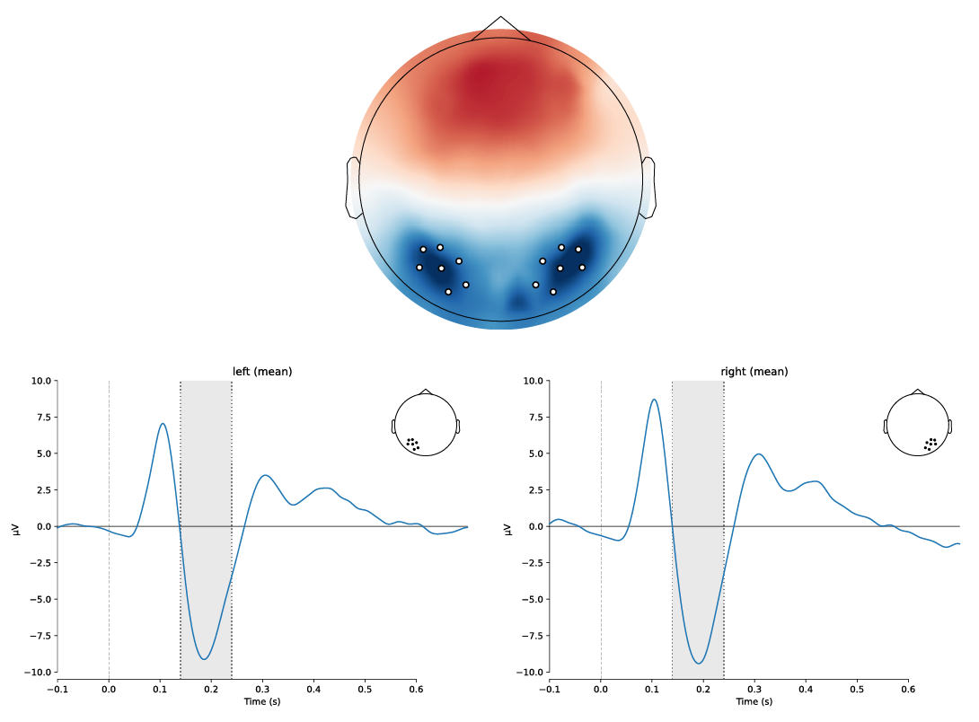
Fig. 13 An example ERP component, the N170. The top panel the distribution of electrical potentials over the scalp (viewed from above, with the nose at the top), averaged over the time period 165-215 ms after stimulus onset. The bottom panels show the time course of the ERP elicited by printed words, averaged over the electrodes indicated by the white dots in the top panel. The vertical line represents stimulus onset, and the shaded grey area indicates the time over which the data were averaged to generate the scalp topographic map. The data are from Galilee et al. (under review).#
As another example, the auditory N1 component is reliably produced by the onset of auditory stimuli; it peaks around 100 ms; it is largest over the midline of the head, anterior to the vertex; and it has negative polarity (i.e., a negative microvolt value). In contrast, the P3 component is elicited by infrequent but task-relevant stimuli; peaks around 300 ms; is largest over the midline posterior region of the scalp, and has positive polarity.
Components are a bit of a strange concept until you get used to them. They are, ultimately, operationally defined and contextually bound. That is to say, if you were given some ERP data without knowing what the stimuli or task were, it would be challenging in most cases to be able to determine what components you were viewing or what the experimental context was that they were recorded in. An expert might be able to distinguish a visual from an auditory experiment, for example, but perhaps not much more than that.
For example, there are numerous other kinds of stimuli besides auditory ones that elicit midline-frontal negativities around 100 ms. As well, the timing and amplitude (size) of ERP components tends to be very sensitive to the precise experimental conditions and parameters (e.g., loudness of an auditory stimulus; brightness and size of a visual stimulus). Identifying and interpreting ERP components thus relies both on knowledge of the existing scientific literature, and of the experiment. That said, given knowledge of the experiment and relevant background literature, ERPs can be a powerful technique for investigating neurocognitive processes. A large number of components have been identified, and associated with particular sensory and cognitive processes. Designing an ERP experiment around particular components can allow the researcher to ask quite nuanced questions about whether, when, and how they occur, and how those processes are modulated by experimental manipulations.
For example, the N1 component elicited by auditory stimuli, mentioned above, can be used in a variety of ways. For one, its amplitude is modulated by attention; attended sounds elicit a larger N1 than unattended sounds. This allows researchers to use the component to investigate many different manipulations of auditory attention. For example, research has shown that auditory attention can be spatially directed, by requiring participants to attend to different spatial locations and playing sounds both from those, and from unattended locations. These studies showed larger N1s in response to stimuli from attended than unattended locations. Moreover, the fact that these effects occurred on the N1, which occurs approximately 100 ms after stimulus onset, allowed insights into the time course of spatially selective attention. Indeed, a common use of ERPs is to identify the earliest point in time at which the brain appears to distinguish between different types of stimuli (or the same stimuli under different contexts).
While in many cases behavioral measures can provide similar insights (e.g., people are faster and more accurate to respond to stimuli at attended than unattended locations, ERP has some advantages over behavioral measures. One advantage is that ERPs do not require any overt response, which means that we can tap into the brain activity involved in a particular aspect of cognitive processing without requiring that the participant think about that process in order to make a response. ERPs also allow us to look at automatic aspects of brain activity, whereas overt behavioral responses necessarily involve conscious decision-making on the part of the participant. Continuing with the auditory attention example, since human motor responses typically take at least 200-250 ms to generate, such measures could not identify 100 ms as the earliest point at which attention modulates stimulus processing. Nor, using only behavioral stimuli, could we know if the requirement to respond to a stimulus was necessary for spatially selective attention to operate. With ERPs, we could compare brain activity on trials where the participant had to respond versus not respond, to address this question.
In most cases it is best to design ERP experiments around particular, expected components, based on a solid understanding of the existing literature on the topic of interest. ERP experiments should be framed in terms of specific hypotheses concerning a particular component or components, how those component(s) will be modulated by the experimental manipulations, and how those modulations of the component(s) will be interpreted, in terms of neurocognitive processes. Typically, “modulation” means differences in amplitude and/or timing (latency) of the component(s) between experimental conditions. In some cases, changes in scalp distribution may also be of interest. Although many components are defined by their scalp distribution, there are a number whose peak location on the scalp differs in meaningful ways. For example, early visual components (such as the P1) differ in their peak location depending on whether the stimulus appears in the left or right, and upper or lower, visual field. This is due to the retinotopic organization of the visual cortex (where the P1 is generated). In other cases, the laterality of a component (whether it is larger over the left or right side of the scalp) may be informative. For example, N170 components are associated with both face processing and word reading, but the face-related N170 tends to be larger over the right hemisphere, whereas the word-related N170 tends to be largest over the left hemisphere (although this is not the case in the example figure above, which is based on data from beginning readers who tend not to show lateralization of the N170 until they get older).