Grand Averages and Visualization#
In this lesson and the next, we’ll work with data from a group of participants, with the aim of testing an experimental hypothesis. The present data do not come from the same experiment as generated the individual participant ERP data we’ve worked with so far. However, they come from another experiment in which an N400 was also predicted. In this experiment, people read sentences that ended in either a semantically congruent word (e.g., I take my coffee with milk and sugar), or an incongruent word (e.g., I take my coffee with milk and glass.). But, similar to the previous experiment, we still predicted an N400 effect, with more negative ERPs for incongruent words than congruent words. Our hypothesis was that there would be a significantly greater negativity, between 400–600 ms, largest over midline central-posterior channels (Cz, CPz, Pz), for incongruent words than congruent words.
The data set comprises preprocessed data files in MNE’s .fif format, one for each participant. The data were preprocessed using the same steps as in the previous lesson, and the data files are named according to the experiment and participant number. For example, the data file for participant 1 is named sentence_n400_p01-ave.fif. Each data set contains data from approximately 80 trials (40 each of Violation and Control) and 64 channels.
The first thing we want to do, when working with ERP data at the group level, is to load in each individual’s preprocessed data, and then calculate the grand average (an average across a group of participants). We will then plot the grand average ERPs, as waveforms and topo plots, to see how the conditions vary at the group level.
Load packages#
import mne
mne.set_log_level('error')  # reduce extraneous MNE output
import matplotlib.pyplot as plt
import numpy as np
import glob
Define parameters#
We define a list of experimental conditions; that’s about the only parameter we need to define here.
conditions = ['Control', 'Violation']
Find data files#
We list all the -ave.fif files (Evoked data sets) associated with this experiment:
data_dir = 'data/group_data/'
data_files = glob.glob(data_dir + 'sentence_n400_p*-ave.fif' )
data_files
['data/group_data/sentence_n400_p22-ave.fif',
 'data/group_data/sentence_n400_p14-ave.fif',
 'data/group_data/sentence_n400_p04-ave.fif',
 'data/group_data/sentence_n400_p05-ave.fif',
 'data/group_data/sentence_n400_p15-ave.fif',
 'data/group_data/sentence_n400_p23-ave.fif',
 'data/group_data/sentence_n400_p17-ave.fif',
 'data/group_data/sentence_n400_p07-ave.fif',
 'data/group_data/sentence_n400_p21-ave.fif',
 'data/group_data/sentence_n400_p20-ave.fif',
 'data/group_data/sentence_n400_p06-ave.fif',
 'data/group_data/sentence_n400_p16-ave.fif',
 'data/group_data/sentence_n400_p13-ave.fif',
 'data/group_data/sentence_n400_p03-ave.fif',
 'data/group_data/sentence_n400_p25-ave.fif',
 'data/group_data/sentence_n400_p24-ave.fif',
 'data/group_data/sentence_n400_p02-ave.fif',
 'data/group_data/sentence_n400_p12-ave.fif',
 'data/group_data/sentence_n400_p26-ave.fif',
 'data/group_data/sentence_n400_p09-ave.fif',
 'data/group_data/sentence_n400_p19-ave.fif',
 'data/group_data/sentence_n400_p10-ave.fif',
 'data/group_data/sentence_n400_p01-ave.fif',
 'data/group_data/sentence_n400_p11-ave.fif',
 'data/group_data/sentence_n400_p18-ave.fif',
 'data/group_data/sentence_n400_p08-ave.fif']
Load data files#
In the previous lesson on averaging trials for an individual participant, we ended by saving the list of MNE Evoked objects (representing the averages across trials for each condition) in a single file for that participant.
Here, we will load in the files from a group of participants. To work with them easily and efficiently in MNE, we will store them as a dictionary, where each key is a condition label, and each value is a list of Evoked objects (the data from that condition, with each participant’s Evoked as a list item).
Here when we read_evokeds() you will likewise get a list of Evoked objects. Lists are a bit tricky since they don’t contain labels. In the previous lesson we addressed this by manually changing the .comment field of each Evoked object to clearly label it. As well, in the case of the present data (as is good practice in any data science pipeline), we used the same code to generate all of the Evoked files, so the two experimental conditions occur in the same order in each -ave.fif file. Since each participant’s data was saved in the same order, index 0 in the list will always be the same condition for all participants. For this reason, we can use enumerate() to loop over conditions and build our dictionary of Evoked objects here.
Note that we use list comprehension to build the list of Evoked objects for each condition, and we use the index from enumerate() (idx) to specify which condition (list item) we read from each participant’s data file:
evokeds = {}

for idx, c in enumerate(conditions):
    evokeds[c] = [mne.read_evokeds(d)[idx].set_montage('easycap-M1') for d in data_files]

evokeds
{'Control': [<Evoked | 'Control' (average, N=40), -0.19922 – 1 s, baseline off, 64 ch, ~387 KiB>,
  <Evoked | 'Control' (average, N=35), -0.19922 – 1 s, baseline off, 64 ch, ~387 KiB>,
  <Evoked | 'Control' (average, N=39), -0.19922 – 1 s, baseline off, 64 ch, ~387 KiB>,
  <Evoked | 'Control' (average, N=38), -0.19922 – 1 s, baseline off, 64 ch, ~387 KiB>,
  <Evoked | 'Control' (average, N=41), -0.19922 – 1 s, baseline off, 64 ch, ~387 KiB>,
  <Evoked | 'Control' (average, N=33), -0.19922 – 1 s, baseline off, 64 ch, ~387 KiB>,
  <Evoked | 'Control' (average, N=40), -0.19922 – 1 s, baseline off, 64 ch, ~387 KiB>,
  <Evoked | 'Control' (average, N=40), -0.19922 – 1 s, baseline off, 64 ch, ~387 KiB>,
  <Evoked | 'Control' (average, N=34), -0.19922 – 1 s, baseline off, 64 ch, ~387 KiB>,
  <Evoked | 'Control' (average, N=40), -0.19922 – 1 s, baseline off, 64 ch, ~387 KiB>,
  <Evoked | 'Control' (average, N=32), -0.19922 – 1 s, baseline off, 64 ch, ~387 KiB>,
  <Evoked | 'Control' (average, N=31), -0.19922 – 1 s, baseline off, 64 ch, ~387 KiB>,
  <Evoked | 'Control' (average, N=10), -0.19922 – 1 s, baseline off, 64 ch, ~387 KiB>,
  <Evoked | 'Control' (average, N=40), -0.19922 – 1 s, baseline off, 64 ch, ~387 KiB>,
  <Evoked | 'Control' (average, N=37), -0.19922 – 1 s, baseline off, 64 ch, ~387 KiB>,
  <Evoked | 'Control' (average, N=35), -0.19922 – 1 s, baseline off, 64 ch, ~387 KiB>,
  <Evoked | 'Control' (average, N=27), -0.19922 – 1 s, baseline off, 64 ch, ~387 KiB>,
  <Evoked | 'Control' (average, N=34), -0.19922 – 1 s, baseline off, 64 ch, ~387 KiB>,
  <Evoked | 'Control' (average, N=39), -0.19922 – 1 s, baseline off, 64 ch, ~387 KiB>,
  <Evoked | 'Control' (average, N=41), -0.19922 – 1 s, baseline off, 64 ch, ~387 KiB>,
  <Evoked | 'Control' (average, N=39), -0.19922 – 1 s, baseline off, 64 ch, ~387 KiB>,
  <Evoked | 'Control' (average, N=39), -0.19922 – 1 s, baseline off, 64 ch, ~387 KiB>,
  <Evoked | 'Control' (average, N=37), -0.19922 – 1 s, baseline off, 64 ch, ~387 KiB>,
  <Evoked | 'Control' (average, N=37), -0.19922 – 1 s, baseline off, 64 ch, ~387 KiB>,
  <Evoked | 'Control' (average, N=41), -0.19922 – 1 s, baseline off, 64 ch, ~387 KiB>,
  <Evoked | 'Control' (average, N=29), -0.19922 – 1 s, baseline off, 64 ch, ~387 KiB>],
 'Violation': [<Evoked | 'Violation' (average, N=40), -0.19922 – 1 s, baseline off, 64 ch, ~387 KiB>,
  <Evoked | 'Violation' (average, N=36), -0.19922 – 1 s, baseline off, 64 ch, ~387 KiB>,
  <Evoked | 'Violation' (average, N=37), -0.19922 – 1 s, baseline off, 64 ch, ~387 KiB>,
  <Evoked | 'Violation' (average, N=38), -0.19922 – 1 s, baseline off, 64 ch, ~387 KiB>,
  <Evoked | 'Violation' (average, N=39), -0.19922 – 1 s, baseline off, 64 ch, ~387 KiB>,
  <Evoked | 'Violation' (average, N=33), -0.19922 – 1 s, baseline off, 64 ch, ~387 KiB>,
  <Evoked | 'Violation' (average, N=34), -0.19922 – 1 s, baseline off, 64 ch, ~387 KiB>,
  <Evoked | 'Violation' (average, N=38), -0.19922 – 1 s, baseline off, 64 ch, ~387 KiB>,
  <Evoked | 'Violation' (average, N=32), -0.19922 – 1 s, baseline off, 64 ch, ~387 KiB>,
  <Evoked | 'Violation' (average, N=39), -0.19922 – 1 s, baseline off, 64 ch, ~387 KiB>,
  <Evoked | 'Violation' (average, N=35), -0.19922 – 1 s, baseline off, 64 ch, ~387 KiB>,
  <Evoked | 'Violation' (average, N=36), -0.19922 – 1 s, baseline off, 64 ch, ~387 KiB>,
  <Evoked | 'Violation' (average, N=10), -0.19922 – 1 s, baseline off, 64 ch, ~387 KiB>,
  <Evoked | 'Violation' (average, N=40), -0.19922 – 1 s, baseline off, 64 ch, ~387 KiB>,
  <Evoked | 'Violation' (average, N=33), -0.19922 – 1 s, baseline off, 64 ch, ~387 KiB>,
  <Evoked | 'Violation' (average, N=26), -0.19922 – 1 s, baseline off, 64 ch, ~387 KiB>,
  <Evoked | 'Violation' (average, N=25), -0.19922 – 1 s, baseline off, 64 ch, ~387 KiB>,
  <Evoked | 'Violation' (average, N=37), -0.19922 – 1 s, baseline off, 64 ch, ~387 KiB>,
  <Evoked | 'Violation' (average, N=38), -0.19922 – 1 s, baseline off, 64 ch, ~387 KiB>,
  <Evoked | 'Violation' (average, N=40), -0.19922 – 1 s, baseline off, 64 ch, ~387 KiB>,
  <Evoked | 'Violation' (average, N=40), -0.19922 – 1 s, baseline off, 64 ch, ~387 KiB>,
  <Evoked | 'Violation' (average, N=39), -0.19922 – 1 s, baseline off, 64 ch, ~387 KiB>,
  <Evoked | 'Violation' (average, N=36), -0.19922 – 1 s, baseline off, 64 ch, ~387 KiB>,
  <Evoked | 'Violation' (average, N=40), -0.19922 – 1 s, baseline off, 64 ch, ~387 KiB>,
  <Evoked | 'Violation' (average, N=38), -0.19922 – 1 s, baseline off, 64 ch, ~387 KiB>,
  <Evoked | 'Violation' (average, N=29), -0.19922 – 1 s, baseline off, 64 ch, ~387 KiB>]}
Compare Evoked waveforms#
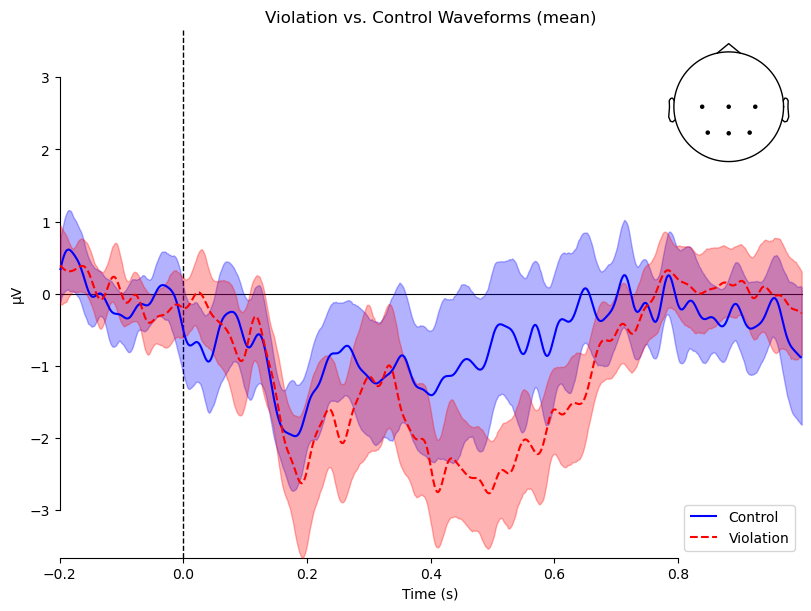
mne.viz.plot_compare_evokeds() will recognize a dictionary of Evoked objects and use the keys as condition labels. Furthermore, when it sees that each value in the dictionary is a list of Evoked objects, it will combine them and plot not only the mean across the list (i.e., across participants, for each condition), but also the 95% confidence intervals (CIs), representing the variability across participants. As we learned in the [EDA] chapter, CIs are a useful way of visually assessing whether different conditions are likely to be statistically significantly different. In this case, the plot shows evidence of an N400 effect. The difference between conditions is largest between ~350–650 ms, and the CIs are most distinct (overlapping little or not at all) between 500–650 ms.
# Define plot parameters
roi = ['C3', 'Cz', 'C4',
       'P3', 'Pz', 'P4']

# set custom line colors and styles
color_dict = {'Control':'blue', 'Violation':'red'}
linestyle_dict = {'Control':'-', 'Violation':'--'}

mne.viz.plot_compare_evokeds(evokeds,
                             combine='mean',
                             legend='lower right',
                             picks=roi, show_sensors='upper right',
                             colors=color_dict,
                             linestyles=linestyle_dict,
                             title='Violation vs. Control Waveforms'
                            )
plt.show()
Differences#
As we did in the single-participant analysis, we can also create difference waves to more easily visualize the difference between conditions, and compare it to zero (i.e., no difference between conditions).
In order to get CIs that reflect the variance across participants, we need to compute the Violation-Control difference separately for each participant. As we did for a single participant’s data, we use mne.combine_evoked() for this, with a weight of 1 for Violation and -1 for Control. The only difference here is we put this function in a list comprehension to loop over participants.
diff_waves = [mne.combine_evoked([evokeds['Violation'][subj],
                                  evokeds['Control'][subj]
                                 ],
                                 weights=[1, -1]
                                 )
              for subj in range(len(data_files))
              ]
diff_waves
[<Evoked | 'Violation - Control' (average, N=20.0), -0.19922 – 1 s, baseline off, 64 ch, ~387 KiB>,
 <Evoked | 'Violation - Control' (average, N=17.74647887323944), -0.19922 – 1 s, baseline off, 64 ch, ~387 KiB>,
 <Evoked | 'Violation - Control' (average, N=18.986842105263158), -0.19922 – 1 s, baseline off, 64 ch, ~387 KiB>,
 <Evoked | 'Violation - Control' (average, N=19.0), -0.19922 – 1 s, baseline off, 64 ch, ~387 KiB>,
 <Evoked | 'Violation - Control' (average, N=19.9875), -0.19922 – 1 s, baseline off, 64 ch, ~387 KiB>,
 <Evoked | 'Violation - Control' (average, N=16.5), -0.19922 – 1 s, baseline off, 64 ch, ~387 KiB>,
 <Evoked | 'Violation - Control' (average, N=18.37837837837838), -0.19922 – 1 s, baseline off, 64 ch, ~387 KiB>,
 <Evoked | 'Violation - Control' (average, N=19.487179487179485), -0.19922 – 1 s, baseline off, 64 ch, ~387 KiB>,
 <Evoked | 'Violation - Control' (average, N=16.484848484848484), -0.19922 – 1 s, baseline off, 64 ch, ~387 KiB>,
 <Evoked | 'Violation - Control' (average, N=19.746835443037973), -0.19922 – 1 s, baseline off, 64 ch, ~387 KiB>,
 <Evoked | 'Violation - Control' (average, N=16.716417910447763), -0.19922 – 1 s, baseline off, 64 ch, ~387 KiB>,
 <Evoked | 'Violation - Control' (average, N=16.65671641791045), -0.19922 – 1 s, baseline off, 64 ch, ~387 KiB>,
 <Evoked | 'Violation - Control' (average, N=5.0), -0.19922 – 1 s, baseline off, 64 ch, ~387 KiB>,
 <Evoked | 'Violation - Control' (average, N=20.0), -0.19922 – 1 s, baseline off, 64 ch, ~387 KiB>,
 <Evoked | 'Violation - Control' (average, N=17.442857142857143), -0.19922 – 1 s, baseline off, 64 ch, ~387 KiB>,
 <Evoked | 'Violation - Control' (average, N=14.918032786885247), -0.19922 – 1 s, baseline off, 64 ch, ~387 KiB>,
 <Evoked | 'Violation - Control' (average, N=12.98076923076923), -0.19922 – 1 s, baseline off, 64 ch, ~387 KiB>,
 <Evoked | 'Violation - Control' (average, N=17.718309859154928), -0.19922 – 1 s, baseline off, 64 ch, ~387 KiB>,
 <Evoked | 'Violation - Control' (average, N=19.246753246753247), -0.19922 – 1 s, baseline off, 64 ch, ~387 KiB>,
 <Evoked | 'Violation - Control' (average, N=20.24691358024691), -0.19922 – 1 s, baseline off, 64 ch, ~387 KiB>,
 <Evoked | 'Violation - Control' (average, N=19.746835443037973), -0.19922 – 1 s, baseline off, 64 ch, ~387 KiB>,
 <Evoked | 'Violation - Control' (average, N=19.5), -0.19922 – 1 s, baseline off, 64 ch, ~387 KiB>,
 <Evoked | 'Violation - Control' (average, N=18.246575342465754), -0.19922 – 1 s, baseline off, 64 ch, ~387 KiB>,
 <Evoked | 'Violation - Control' (average, N=19.22077922077922), -0.19922 – 1 s, baseline off, 64 ch, ~387 KiB>,
 <Evoked | 'Violation - Control' (average, N=19.72151898734177), -0.19922 – 1 s, baseline off, 64 ch, ~387 KiB>,
 <Evoked | 'Violation - Control' (average, N=14.5), -0.19922 – 1 s, baseline off, 64 ch, ~387 KiB>]
Plot difference waveform#
In making the difference waveform above, we simply created a list of Evoked objects. We didn’t create a dictionary since there is only one contrast (Violation-Control), so no need to have informative dictionary keys for a set of different items (contrasts). This is fine, however MNE’s plot_compare_evokeds() has some complicated behavior when it comes to its inputs, and whether it draws CIs or not. Specifically, the API reads:
If a list of Evokeds, the contents are plotted with their .comment attributes used as condition labels… If a dict whose values are Evoked objects, the contents are plotted as single time series each and the keys are used as labels. If a [dict/list] of lists, the unweighted mean is plotted as a time series and the parametric confidence interval is plotted as a shaded area.
In other words, when the function gets a list of Evoked objects as input, it will draw each object as a separate waveform, but if it gets a dictionary in which each entry is a list of Evoked objects, if will average them together and draw CIs. Since we desire the latter behavior here, in the command below we create a dictionary “on the fly” inside the plotting command, with a key corresponding to the label we want, and the value being the list of difference waves.
contrast = 'Violation-Control'
mne.viz.plot_compare_evokeds({contrast:diff_waves}, combine='mean',
                            legend=None,
                            picks=roi, show_sensors='upper right',
                            title=contrast
                            )
plt.show()
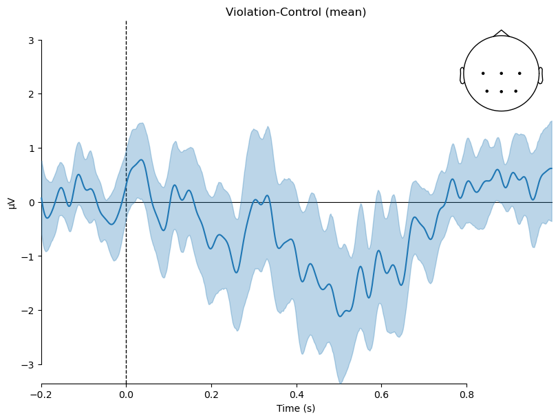
The nice thing about 95% CIs is that they provide an easy visual aid for interpreting the results. If the CI overlaps zero, then the difference between conditions is not statistically significant. If the CI does not overlap zero, then the difference can be considered statistically significant. In this case, the CI largely does not overlap zero between ~400–600 ms, so we can conclude that the difference between conditions is statistically significant in that time window.
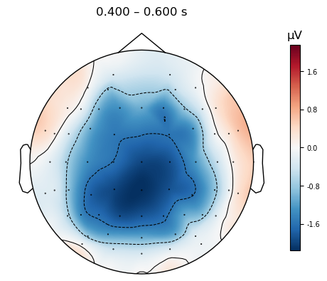
Scalp topographic map#
As with plot_compare_evoked(), it’s important to understand what type of data the plot_evoked_topomap() function needs in order to get it to work right. Whereas plot_compare_evoked() will average over a list of Evoked objects, plot_evoked_topomap() will only accept a single Evoked object as input. Therefore, in the command below we apply the mne.grand_average() function to the list of Evoked objects (Grand averaging is a term used in EEG research to refer to an average across participants; this terminology developed to distinguish such an average from an average across trials, for a single participant).
Here we plot the topographic map for the average amplitude over a 200 ms period, centered on 400 ms (i.e., 300–500 ms).
mne.viz.plot_evoked_topomap(mne.grand_average(diff_waves),
                            times=.500, average=0.200,
                            size=3
                           )
plt.show()
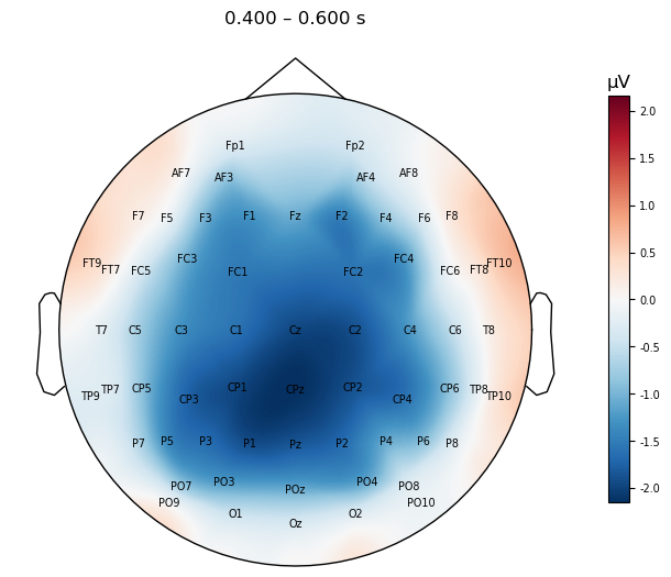
We can add a few enhancements to the plot to make it more interpretable:
The
show_nameskwarg tells the function to plot the names of each channel. We also usesensors=Falseotherwise the dots for each channel would overlap the names.The
contours=Falsekwarg turns off the dashed contour lines you can see above. This is a matter of personal preference, however I feel that these are like non-continuous colour scales, in that they provide visual indicators of discontinuous “steps” in the scalp electrical potential values, when in fact these vary smoothly and continuously.We increase the
sizeto make the channel labels a bit easier to read (unfortunately the function doesn’t provide a kwarg to adjust the font size of these).
mne.viz.plot_evoked_topomap(mne.grand_average(diff_waves),
                            times=.500, average=0.200,
                            show_names=True, sensors=False,
                            contours=False,
                            size=4
                           );
Summary#
In this lesson we learned how to load in a group of Evoked objects, and how to use MNE’s plot_compare_evokeds() function to plot the average waveforms for each condition, and the 95% confidence intervals (CIs) for each. We also learned how to create difference waves, and plot the average difference wave with CIs. Finally, we learned how to plot a scalp topographic map of the average amplitude over a time window of interest. Of course, none of this tells us whether the Violation–Control difference is statistically significant. We will learn how to do that in the next lesson.