Visualizing Raw EEG using MNE#
In this section we will see how to plot various attributes of a raw EEG data file using functions and methods provided by the MNE library. THis includes viewing data over time, over the scalp, and also plotting electrode locations on the scalp. We will use the same data file that we used in the previous section.
import mne
mne.set_log_level('error')

import numpy as np
import matplotlib.pyplot as plt

raw = mne.io.read_raw_brainvision('data/sub-001/sub-001.vhdr',
                                  preload=True)
Descriptive statistics on channels#
We saw preivously how to get metadata from the raw file using the .info property. Another useful way of peeking into a raw file’s data is to use the .describe() method to see the names of each channel, and the range of values in each channel.
raw.describe()
<RawBrainVision | sub-001.eeg, 16 x 408640 (817.3 s), ~49.9 MiB, data loaded>
ch  name  type  unit        min         Q1     median         Q3        max
 0  Fp1   EEG   µV      -285.40     -30.22      -1.43      27.83    1301.03
 1  F3    EEG   µV      -174.79     -17.23       9.22      27.46     253.16
 2  F7    EEG   µV      -218.86     -27.54       1.24      27.61     840.83
 3  C3    EEG   µV      -143.89     -11.69       2.93      14.49     125.35
 4  P3    EEG   µV      -222.93     -16.64       1.79      19.13      98.77
 5  TP9   EEG   µV      -521.95     -24.35      10.94      48.68     507.04
 6  Fz    EEG   µV       -63.42     -10.49      -0.49      12.11      96.25
 7  Cz    EEG   µV      -122.98     -16.84      -0.59      16.92      70.10
 8  Fp2   EEG   µV      -308.07     -34.05       0.94      32.26     455.79
 9  F4    EEG   µV       -88.54     -11.64       3.62      14.80     123.72
10  F8    EEG   µV      -390.29     -19.68      -0.60      14.91     241.88
11  C4    EEG   µV      -166.15     -21.28       1.28      19.47     104.65
12  P4    EEG   µV      -375.89     -21.70       0.88      30.19     201.16
13  TP10  EEG   µV      -236.19     -21.82       0.85      21.64     388.90
14  Pz    EEG   µV      -165.69     -12.59       3.75      17.90      76.89
15  Oz    EEG   µV      -229.21     -15.15       5.89      24.40     194.92
Set Montage#
The raw file contains the 10-20 system labels for each channel, but it doesn’t provide information about the location of each electrode on the scalp. Internally, MNE can represent the location of each channel in a 3D Cartesian coordinate system. This is necessary to plot the locations of the channels on the scalp, which is extremely useful when visualizing EEG data. The set of coordinates for each channel is called the montage of the raw file. We can set the montage of the raw file to the 10-20 system using the set_montage() method. This will add the location information to the raw file. MNE provies a large set of standard montages for many commercial EEG systems. For the present data, the EEG caps were manufactured by a company named Easycap, and so we load the montage for the Easycap system.
raw.set_montage('easycap-M1')
| General | ||
|---|---|---|
| Filename(s) | sub-001.eeg | |
| MNE object type | RawBrainVision | |
| Measurement date | 2015-01-20 at 13:15:58 UTC | |
| Participant | Unknown | |
| Experimenter | Unknown | |
| Acquisition | ||
| Duration | 00:13:38 (HH:MM:SS) | |
| Sampling frequency | 500.00 Hz | |
| Time points | 408,640 | |
| Channels | ||
| EEG | ||
| Head & sensor digitization | 19 points | |
| Filters | ||
| Highpass | 0.01 Hz | |
| Lowpass | 80.00 Hz | |
The coordinates for each location are stored in the 'dig' attribute of the info object. The dig attribute is a list of objects of the MNE type mne.io._digitization.DigPoint. Each electrode location is stored as a set of (x, y, z) Cartesian coordinates, i.e., positions in a 3D grid, where x is the left-right dimension, y is posterior-anterior, and z is inferior-posterior. The (0, 0, 0) location is inside the head, located in a plane defined by the bridge of the nose (called the nasion) and the left and right ear canals. As shown in the figure below, x goes from left (negative) to right (positive), y goes from posterior to anterior, and z goes from inferior to superior. In general, you won’t need to work with this coordinate system directly, but it’s useful to know how the data are represented.
raw.info['dig']
[<DigPoint |        LPA : (-86.1, -0.0, 0.0) mm     : head frame>,
 <DigPoint |     Nasion : (0.0, 86.1, 0.0) mm       : head frame>,
 <DigPoint |        RPA : (86.1, 0.0, 0.0) mm       : head frame>,
 <DigPoint |     EEG #1 : (-29.3, 90.3, 36.8) mm    : head frame>,
 <DigPoint |     EEG #2 : (29.3, 90.3, 36.8) mm     : head frame>,
 <DigPoint |     EEG #3 : (-51.8, 63.9, 87.6) mm    : head frame>,
 <DigPoint |     EEG #4 : (51.8, 63.9, 87.6) mm     : head frame>,
 <DigPoint |     EEG #5 : (-68.3, -0.0, 106.1) mm   : head frame>,
 <DigPoint |     EEG #6 : (68.3, 0.0, 106.1) mm     : head frame>,
 <DigPoint |     EEG #7 : (-51.8, -63.9, 87.6) mm   : head frame>,
 <DigPoint |     EEG #8 : (51.8, -63.9, 87.6) mm    : head frame>,
 <DigPoint |    EEG #11 : (-76.8, 55.8, 36.8) mm    : head frame>,
 <DigPoint |    EEG #12 : (76.8, 55.8, 36.8) mm     : head frame>,
 <DigPoint |    EEG #17 : (0.0, 68.3, 106.1) mm     : head frame>,
 <DigPoint |    EEG #18 : (0.0, 0.0, 135.1) mm      : head frame>,
 <DigPoint |    EEG #19 : (0.0, -68.3, 106.1) mm    : head frame>,
 <DigPoint |    EEG #60 : (-81.9, -26.6, 0.0) mm    : head frame>,
 <DigPoint |    EEG #61 : (81.9, -26.6, 0.0) mm     : head frame>,
 <DigPoint |    EEG #73 : (0.0, -94.9, 36.8) mm     : head frame>]
Note above that the list of sensor locations does not contain the names of each sensor — the channel names we saw above. In general MNE’s data structures are designed to assume that channels are listed in the same order in all attributes of the data structure. So, the order of labels in the list of channel names from raw.info['ch_names'] corresponds to the order of the channel locations in raw.info['dig'].
raw.info['ch_names']
['Fp1',
 'F3',
 'F7',
 'C3',
 'P3',
 'TP9',
 'Fz',
 'Cz',
 'Fp2',
 'F4',
 'F8',
 'C4',
 'P4',
 'TP10',
 'Pz',
 'Oz']
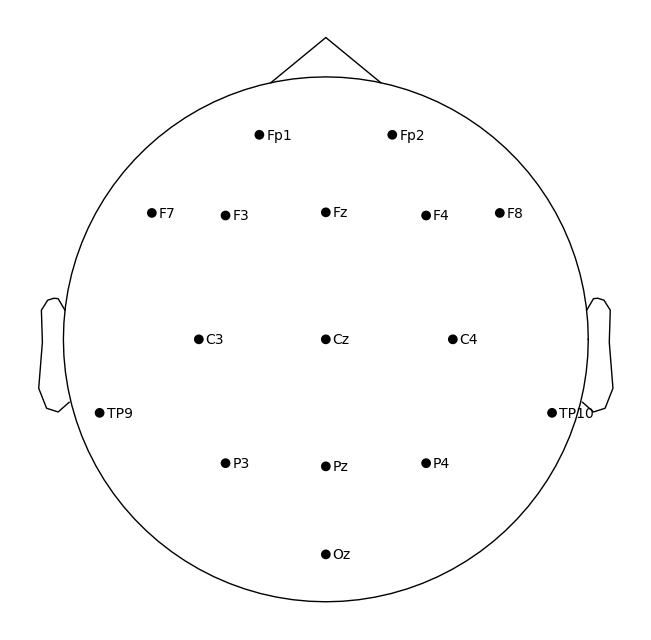
View electrode positions#
MNE provides tools for viewing channel locations in both 2D and 3D.
Tip
Always remember to use plt.show(), or put a semicolon after an MNE plot command. Otherwise the plot will be drawn twice.
raw.plot_sensors(show_names=True)
plt.show()
Interactive Plot of Continuous EEG#
We could add more code to the above cell to do things like label the axes, add a title to indicate what electrode the data came from, make the x axis actually represent units of time, etc.. However, the great value of using MNE is that the developers have created customized functions for doing most everything you could ever want with EEG, with a lot less typing that if you were working with raw NumPy arrays and Matplotlib.
For example, MNE data classes like Raw have a .plot method that allows you to generate a nice-looking plot that automatically does all the hard work of formatting it appropriately. This function actually creates an interactive plot in a new window (which is why you won’t see output in this notebook file), which allows you to scroll through the entire continuous dataset (unfortunately this doesn’t work if you’re running Jupyter notebooks via a cloud service, but should work fine if you followed the instructions at the start of this course and are using VS Code).
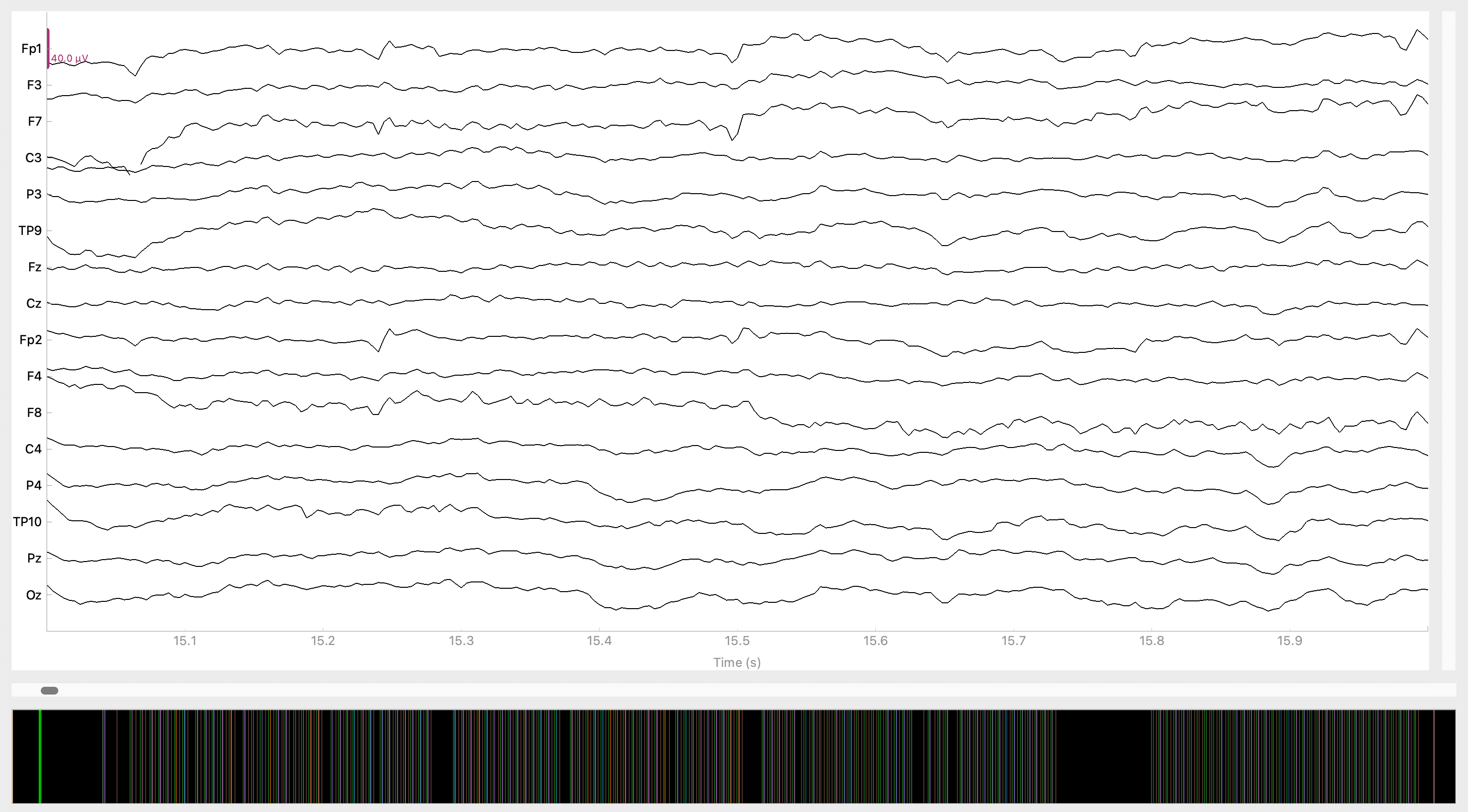
The black area at the bottom shows the entire raw EEG recording, with a green vertical bar near the start indicating the position in the file that is currently plotted, and a drag bar to scroll through the data. The other colored vertical lines mark the times of event codes sent by the stimulus presentation program, which mark events of experimental interest.
Event codes (Markers / Triggers)#
Event codes — often called markers or triggers are codes that are sent by the stimulus presentation program to mark the times of events of experimental interest. The event codes are stored in the .vmrk file in Brain Vision format. When we import the raw data into MNE, these are stored in an attribute called ._annotations. Although we can access that directly (e.g., raw._annotations), again MNE provides tools that makes this easier and generate more interpretable output: the events_from_annotations() function:
mne.events_from_annotations(raw)
(array([[     0,      0,  10001],
        [ 25550,      0,      5],
        [ 25553,      0,      1],
        ...,
        [397701,      0,      3],
        [402068,      0,      7],
        [402073,      0,      4]], shape=(532, 3)),
 {np.str_('Comment/actiCAP Data On'): 10001,
  np.str_('Stimulus/S  1'): 1,
  np.str_('Stimulus/S  2'): 2,
  np.str_('Stimulus/S  3'): 3,
  np.str_('Stimulus/S  4'): 4,
  np.str_('Stimulus/S  5'): 5,
  np.str_('Stimulus/S  7'): 7,
  np.str_('Stimulus/S101'): 101,
  np.str_('Stimulus/S102'): 102,
  np.str_('Stimulus/S111'): 111,
  np.str_('Stimulus/S112'): 112,
  np.str_('Stimulus/S201'): 201,
  np.str_('Stimulus/S202'): 202,
  np.str_('Stimulus/S211'): 211,
  np.str_('Stimulus/S212'): 212})
The result includes two outputs. The first is a NumPy array that has three columns, with one row for each event code in the data. The first column indicates the time of the event, and the last column stores the code associated with that event. These event codes are always represented as integers (since it is a NumPy array of integers).
The second output is a dictionary mapping labels for each event code, to the numerical codes themselves. Usually these are not very informative in the raw data. In a later lesson, we will learn how to map the numerical codes to meaningful labels based on the experimental design. For now, it’s simply important to understand how the event codes are stored in the Raw data object.
One important thing to know is that the event codes are stored in the same units as the data, so in this case, the event codes are in units of samples, not milliseconds. MNE knows this and operates accordingly, but if you want to know the time of an event in milliseconds, you need to convert it yourself based on the sampling rate. In this case, our sampling rate is 500 Hz, if we wanted to see the event timings in milliseconds we can divide the event time by the sampling rate, and multiplying by 1000. We can do this below by first assigning the two outputs of mne.events_from_annotations() to two variables, and then converting the values in the first column of the events `array`` to milliseconds:
events, event_dict = mne.events_from_annotations(raw)

# MNE expects the events array in terms of samples, so don't change it
# Create a copy of the events array and convert the first column to ms
events_ms = events.copy()
events_ms[:, 0] = events_ms[:, 0] / 500 * 1000
events_ms[:10]
array([[    0,     0, 10001],
       [51100,     0,     5],
       [51106,     0,     1],
       [52198,     0,   201],
       [52288,     0,     2],
       [59164,     0,     3],
       [66566,     0,     1],
       [67562,     0,   211],
       [69864,     0,     3],
       [72286,     0,     1]])
Again, it’s generally better to work with MNE objects using MNE’s own functions and methods, but sometimes it’s important to understand the events array. For example, there may be circumstances when you need to modify event codes. For example, we might want to separately average trials on which participants made correct and incorrect responses. In that case, we would need to change the event codes for stimuli followed by incorrect responses to something different than the event codes for correct responses.
raw.describe()
<RawBrainVision | sub-001.eeg, 16 x 408640 (817.3 s), ~49.9 MiB, data loaded>
ch  name  type  unit        min         Q1     median         Q3        max
 0  Fp1   EEG   µV      -285.40     -30.22      -1.43      27.83    1301.03
 1  F3    EEG   µV      -174.79     -17.23       9.22      27.46     253.16
 2  F7    EEG   µV      -218.86     -27.54       1.24      27.61     840.83
 3  C3    EEG   µV      -143.89     -11.69       2.93      14.49     125.35
 4  P3    EEG   µV      -222.93     -16.64       1.79      19.13      98.77
 5  TP9   EEG   µV      -521.95     -24.35      10.94      48.68     507.04
 6  Fz    EEG   µV       -63.42     -10.49      -0.49      12.11      96.25
 7  Cz    EEG   µV      -122.98     -16.84      -0.59      16.92      70.10
 8  Fp2   EEG   µV      -308.07     -34.05       0.94      32.26     455.79
 9  F4    EEG   µV       -88.54     -11.64       3.62      14.80     123.72
10  F8    EEG   µV      -390.29     -19.68      -0.60      14.91     241.88
11  C4    EEG   µV      -166.15     -21.28       1.28      19.47     104.65
12  P4    EEG   µV      -375.89     -21.70       0.88      30.19     201.16
13  TP10  EEG   µV      -236.19     -21.82       0.85      21.64     388.90
14  Pz    EEG   µV      -165.69     -12.59       3.75      17.90      76.89
15  Oz    EEG   µV      -229.21     -15.15       5.89      24.40     194.92
Summary#
MNE Provides a number of methods for Raw objects that allow us to access and visualize aspects of both the metadata — including channel locations — and the data itself. However, in practice these are useful things to be familiar with, and they can be used when you’re working with data from a system or format that you’re not familiar with to get a better idea of the structure of the data. But in routine usage, within the context of a specific experiment we can expect that all of the data have the same structure. In the next series of lessons we’ll walk through the steps that are routinely applied to any EEG data set, in order to prepare it for ERP analysis.